In graph theory , reachability refers to the ability to get from one vertex to another within a graph. A vertex s {\displaystyle s} can reach a vertex t {\displaystyle t} (and t...
Worldlex WikiFrancaisLecture gratuite
In graph theory, reachability refers to the ability to get from one vertex to another within a graph. A vertex
In an undirected graph, reachability between all pairs of vertices can be determined by identifying the connected components of the graph. Any pair of vertices in such a graph can reach each other if and only if they belong to the same connected component; therefore, in such a graph, reachability is symmetric ( reaches iff reaches ). The connected components of an undirected graph can be identified in linear time. The remainder of this article focuses on the more difficult problem of determining pairwise reachability in a directed graph (which, incidentally, need not be symmetric).
Definition
For a directed graph , with vertex set and edge set , the reachability relation of is the transitive closure of , which is to say the set of all ordered pairs of vertices in for which there exists a sequence of vertices such that the edge is in for all .
If is acyclic, then its reachability relation is a partial order; any partial order may be defined in this way, for instance as the reachability relation of its transitive reduction. A noteworthy consequence of this is that since partial orders are anti-symmetric, if can reach , then we know that cannot reach . Intuitively, if we could travel from to and back to , then would contain a cycle, contradicting that it is acyclic. If is directed but not acyclic (i.e. it contains at least one cycle), then its reachability relation will correspond to a preorder instead of a partial order.
Algorithms
Algorithms for determining reachability fall into two classes: those that require preprocessing and those that do not.
If you have only one (or a few) queries to make, it may be more efficient to forgo the use of more complex data structures and compute the reachability of the desired pair directly. This can be accomplished in linear time using algorithms such as breadth first search or iterative deepening depth-first search.
If you will be making many queries, then a more sophisticated method may be used; the exact choice of method depends on the nature of the graph being analysed. In exchange for preprocessing time and some extra storage space, we can create a data structure which can then answer reachability queries on any pair of vertices in as low as time. Three different algorithms and data structures for three different, increasingly specialized situations are outlined below.
Floyd–Warshall Algorithm
The Floyd–Warshall algorithm can be used to compute the transitive closure of any directed graph, which gives rise to the reachability relation as in the definition, above.
The algorithm requires time and space in the worst case. This algorithm is not solely interested in reachability as it also computes the shortest path distance between all pairs of vertices. For graphs containing negative cycles, shortest paths may be undefined, but reachability between pairs can still be noted.
Thorup's Algorithm
For planardigraphs, a much faster method is available, as described by Mikkel Thorup in 2004. This method can answer reachability queries on a planar graph in time after spending preprocessing time to create a data structure of size. This algorithm can also supply approximate shortest path distances, as well as route information.
The overall approach is to associate with each vertex a relatively small set of so-called separator paths such that any path from a vertex to any other vertex must go through at least one of the separators associated with or . An outline of the reachability related sections follows.
Given a graph , the algorithm begins by organizing the vertices into layers starting from an arbitrary vertex . The layers are built in alternating steps by first considering all vertices reachable from the previous step (starting with just ) and then all vertices which reach to the previous step until all vertices have been assigned to a layer. By construction of the layers, every vertex appears at most two layers, and every directed path, or dipath, in is contained within two adjacent layers and . Let be the last layer created, that is, the lowest value for such that .
The graph is then re-expressed as a series of digraphs where each and where is the contraction of all previous levels into a single vertex. Because every dipath appears in at most two consecutive layers, and because each is formed by two consecutive layers, every dipath in appears in its entirety in at least one (and no more than 2 consecutive such graphs)
For each , three separators are identified which, when removed, break the graph into three components which each contain at most the vertices of the original. As is built from two layers of opposed dipaths, each separator may consist of up to 2 dipaths, for a total of up to 6 dipaths over all of the separators. Let be this set of dipaths. The proof that such separators can always be found is related to the Planar Separator Theorem of Lipton and Tarjan, and these separators can be located in linear time.
For each , the directed nature of provides for a natural indexing of its vertices from the start to the end of the path. For each vertex in , we locate the first vertex in reachable by , and the last vertex in that reaches to . That is, we are looking at how early into we can get from , and how far we can stay in and still get back to . This information is stored with each . Then for any pair of vertices and , can reach via if connects to earlier than connects from .
Every vertex is labelled as above for each step of the recursion which builds . As this recursion has logarithmic depth, a total of extra information is stored per vertex. From this point, a logarithmic time query for reachability is as simple as looking over each pair of labels for a common, suitable . The original paper then works to tune the query time down to .
In summarizing the analysis of this method, first consider that the layering approach partitions the vertices so that each vertex is considered only times. The separator phase of the algorithm breaks the graph into components which are at most the size of the original graph, resulting in a logarithmic recursion depth. At each level of the recursion, only linear work is needed to identify the separators as well as the connections possible between vertices. The overall result is preprocessing time with only additional information stored for each vertex.
Kameda's Algorithm
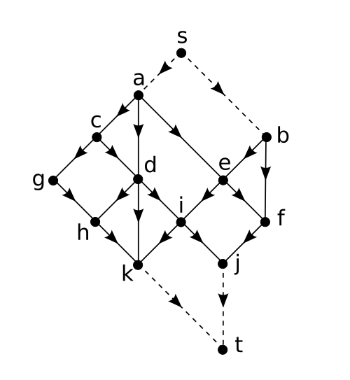
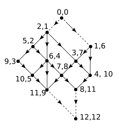
A suitable digraph for Kameda's method with and added.The same graph as above after Kameda's algorithm has run, showing the DFS labels for each vertex
An even faster method for pre-processing, due to T. Kameda in 1975, can be used if the graph is planar, acyclic, and also exhibits the following additional properties: all 0-indegree and all 0-outdegree vertices appear on the same face (often assumed to be the outer face), and it is possible to partition the boundary of that face into two parts such that all 0-indegree vertices appear on one part, and all 0-outdegree vertices appear on the other (i.e. the two types of vertices do not alternate).
If exhibits these properties, then we can preprocess the graph in only time, and store only extra bits per vertex, answering reachability queries for any pair of vertices in le temps avec une simple comparaison.
Le prétraitement effectue les étapes suivantes. Nous ajoutons un nouveau sommet.qui possède une arête vers chaque sommet de degré entrant 0, et un autre nouveau sommetavec des arêtes issues de chaque sommet de degré sortant nul. Notez que les propriétés deCela nous permet de procéder tout en préservant la planarité, c'est-à-dire qu'il n'y aura toujours pas d'intersections d'arêtes après ces ajouts. Pour chaque sommet, nous stockons la liste des adjacences (arêtes sortantes) selon l'ordre de planarité du graphe (par exemple, dans le sens horaire par rapport à l'immersion du graphe). Nous initialisons ensuite un compteur.et commencer un parcours en profondeur à partir deLors de ce parcours, la liste d'adjacence de chaque sommet est visitée de gauche à droite, selon les besoins. Au fur et à mesure que les sommets sont retirés de la pile de parcours, ils sont étiquetés avec la valeur, etest ensuite décrémenté. Notez queest toujours étiqueté avec la valeuretest toujours étiqueté avecLe parcours en profondeur est ensuite répété, mais cette fois-ci la liste d'adjacence de chaque sommet est visitée de droite à gauche.
Une fois terminé,etLes sommets et leurs arêtes incidentes sont supprimés. Chaque sommet restant stocke une étiquette bidimensionnelle avec des valeurs issues deàÉtant donné deux sommetsetet leurs étiquetteset, nous disons quesi et seulement si,, et il existe au moins un composantouce qui est strictement inférieur àou, respectivement.
Le principal résultat de cette méthode est donc queest accessible depuissi et seulement si, ce qui se calcule facilement danstemps.
Problèmes connexes
Un problème connexe consiste à résoudre les requêtes d'accessibilité avec un certain nombredes défaillances de sommets. Par exemple : « Peut-on avoir un sommetatteindre encore le sommetmême si les sommets« Ont échoué et ne peuvent plus être utilisés ? » Un problème similaire peut considérer les défaillances d’arêtes plutôt que les défaillances de sommets, ou une combinaison des deux. La technique de recherche en largeur fonctionne tout aussi bien sur de telles requêtes, mais la construction d’un oracle efficace est plus complexe.
Un autre problème lié aux requêtes d'accessibilité concerne le recalcul rapide des relations d'accessibilité lorsqu'une partie du graphe est modifiée. Par exemple, cela pose un problème important pour le ramasse-miettes , qui doit trouver un équilibre entre la récupération de la mémoire (afin qu'elle puisse être réallouée) et les impératifs de performance de l'application en cours d'exécution.